Drawing Graphs with Circular Vertices

Graph drawing is a common algorithmical problem applicable to many fields besides software; common examples include the analysis of social networks or the visualization of biological graphs. In this article, I describe a simple extension to a standard force-directed algorithm that allows to draw graphs with circular vertices.

Force-directed algorithms or spring embedders place vertices by assigning forces according to the edges connecting the vertices. These algorithms are intuitive, able to yield solutions of high quality in a reasonable amount of time and can be applied to most kinds of graphs. For conciseness, most fundamentals will be omitted, a basic knowledge of these kind of algorithms is presumed.

Original algorithm

We employ a standard force-directed algorithm as a basis, that is, the algorithm of Fruchterman and Reingold. It assumes vertices to be point-shaped and defines two forces for influencing vertices: An attractive force f_attr that pulls connected vertices towards each other and a repulsive force f_rep that disperses the vertices by repelling them from each other. The absolute value of the forces can be computed as follows:

• f_attr(u, v) = k² / distance(u, v)
• f_rep(u, v) = distance(u, v)² / k

The directions of the forces are determined from the positions of the vertices given as two-dimensional vectors; for two vertices, the direction of repulsion and attraction is inverse. The complete force affecting a vertex v is computed by adding the repulsive forces for all other vertices and the attractive forces for all connected vertices together. As shown in the following figure, k describes the distance between two connected vertices whose attractive and repulsive forces are in equilibrium.

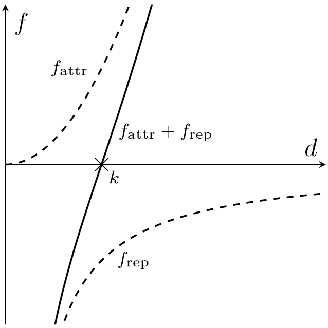
The factor k is a constant and usually chosen according to the area of the drawing. If the distance between two vertices shrinks towards zero, the repulsive force grows infinitely. Similarly, for two connected vertices the attractive force grows with the distance between them. More information about the original algorithm can be found in the paper “Graph Drawing by Force-directed Placement“.

This approach works fine for point-shaped vertices, however, it cannot deal with two-dimensional vertices: It cannot ensure that vertices do not overlap, but only prevents their centers from touching. Next, I will present a slight modification of the algorithm in order to enable the handling of circular vertices.

Modified algorithm

Our goal is to ensure a minimum distance between all vertices so that their borders can neither touch nor overlap. Additionally, in contrast to the original algorithm where the distance between vertices depends on a constant, the distance of vertices should be determined according to the size of the vertices, that is, smaller vertices may be placed more near to each other than larger vertices.

As illustrated in the next figure, one way to meet the first requirement is to adjust the force functions. If the repulsive force grows infinitely when dwindling to a certain distance, this distance poses a lower bound for the distance of two vertices.

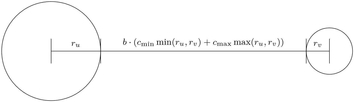
Furthermore, in order to fulfill the second requirement, the minimum and preferred distance functions are parameterized with the radii of the vertices as follows:

• d_min(u, v) = r_u + r_v + b_min · (c_min min(r_u, r_v) + c_max max(r_u, r_v))
• d_pref(u, v) = r_u + r_v + b_pref · (c_min min(r_u, r_v) + c_max max(r_u, r_v))

The addition of the radii r_u and r_v ensures that vertices corresponding to the minimum distance never overlap. The constant b_x controls the size of the buffer between two vertices subject to their radii as shown in the figure below. Finally, the constants c_min and c_max weigh the influence of the radii; this allows us to place a small vertex more near to a large vertex than another large vertex. The factors b_x, c_min and c_max should be positive and c_min and c_max should add up to one.

On this basis the force functions can be redefined. Let d_actual(u, v) be the actual distance between two vertices u and v and let d‘_X(u, v) be the distance normalized by the minimum distance:

• d_actual(u, v) = |pos(v) – pos(u)|
• d‘_X(u, v) = d_X(u, v) – d_min(u, v)

This results in the following force functions, which comply with the criteria specified before:

Finally, this leads us to the pseudocode of the complete algorithm for layouting a graph G = (V, E):

procedure Layout(G = (V, E))
    initialize temperature t
    for i = 1 to n do
        for each v in V do
            disp(v) = 0
            for each u in V do
                if u ≠ v then
                    Δ = pos(v) - pos(u)
                    disp(v) = disp(v) + Δ/|Δ| · f_rep(u, v)
        for each (u, v) in E do
            Δ = pos(v) - pos(u)
            disp(v) = disp(v) - Δ/|Δ| · f_attr(u, v)
            disp(u) = disp(u) + Δ/|Δ| · f_attr(u, v)
        for each v in V do
            pos(v) = pos(v) + disp(v)/|disp(v)| · min(|disp(v)|, t)
        t = cool(t)

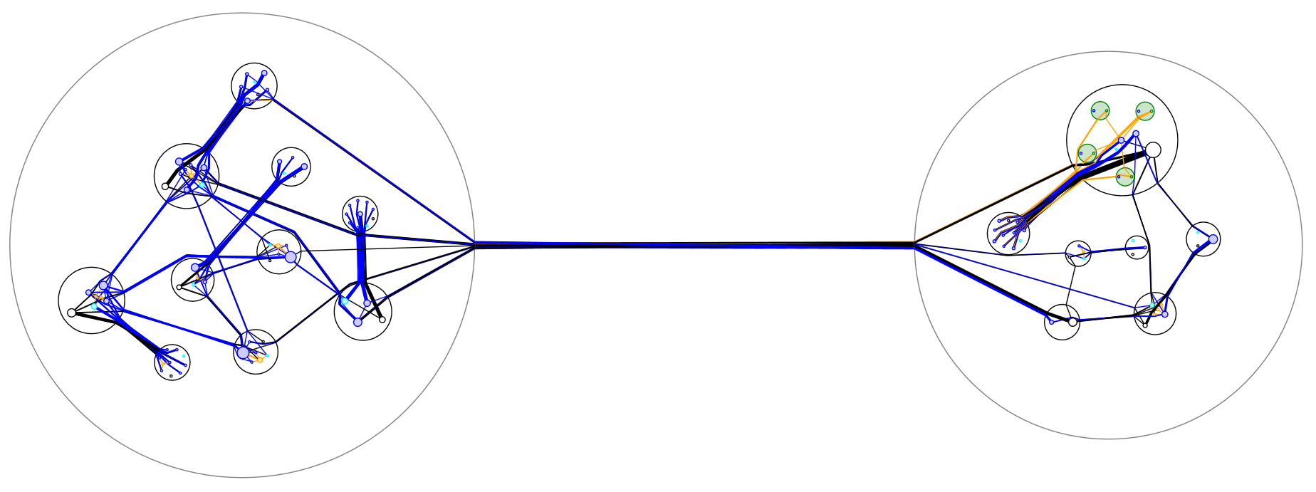
Applications

The drawings produced by this algorithm are not perfect, however, it is possible to employ it in a more complex context. For example, we used it to visualize the structure of software; an example can be seen in the figure below. The techniques behind this other layout algorithm are described in detail here.